Multilayer Perceptron in Machine Learning: Machine learning is full of terms that sometimes feel abstract. Among them, multilayer perceptron in machine learning is one of the foundational models in neural networks.

In this blog, we will explore what is multilayer perceptron, how it differs from simpler models, how it learns (especially back propagation in multilayer perceptrons), and even how it can implement logic functions like xor gate using multilayer perceptron.

We will also touch upon advanced variants like extreme learning machine for multilayer perceptron, and see diagram of multilayer perceptron to visualise the architecture. By the end, you should have a clear understanding of multilayer perceptron in machine learning.

Why Multilayer Perceptron?

Suppose you want to classify images, or predict non-linear relationships (e.g. house price from many features). Simple models like linear regression or a single perceptron (i.e. one layer) often struggle because they can only form linear separations. That is where multilayer perceptron in machine learning enters: it allows modelling of non-linear decision boundaries.

You might ask: Why not just use a single layer perceptron with clever weights? The answer is: if the data is not linearly separable, no weighting of a single layer can split the classes correctly. Classic example would be – XOR. A single perceptron fails on XOR, but a multilayer perceptron in machine learning with hidden layers succeeds.

In short: multilayer perceptron in machine learning gives us expressive power to learn non-linear mappings that simple linear models or single perceptrons can’t.

What Is Multilayer Perceptron in Machine Learning?

So, what is multilayer perceptron exactly? Well, a multilayer perceptron (MLP), which is what we mean by multilayer perceptron in machine learning is a feedforward artificial neural network with at least three layers:

• An input layer (receiving features)
• One or more hidden layers
• An output layer

Each neuron (node) in one layer is connected (via weighted edges) to every neuron in the next layer (fully connected). The neurons use a nonlinear activation function (e.g. sigmoid, tanh, ReLU) so that the network can approximate non-linear functions.

In formal terms, an MLP is a feedforward neural network: data moves in one direction (input > hidden > output) with no cycles.

A multilayer perceptron (MLP) is a modern feedforward neural network consisting of fully connected neurons with nonlinear activation functions, organized in layers. Thus, when you read multilayer perceptron in machine learning, think of a multi-layer network that can learn complex mappings beyond linear.

Difference Between Single Layer and Multilayer Perceptron

It helps to contrast and see the difference between single layer and multilayer perceptron:

Aspects	Single Layer Perceptron	Multilayer Perceptron
Layers	Only input + output (no hidden layers)	Input + one or more hidden + output
Representational power	Can only solve linearly separable problems	Can solve non-linear problems
Activation	Often step / threshold function	Uses differentiable nonlinear activations (sigmoid, ReLU etc.)
Learning algorithm	Perceptron learning rule (simple)	Uses back propagation in multilayer perceptrons (gradient descent)
Limitations	Cannot learn XOR, cannot model complex boundaries	More powerful but more complexity, risk of overfitting

Because of this, the single layer perceptron is insufficient when your data requires non-linear separation. The difference between single layer and multilayer perceptron is that the multilayer version introduces hidden layers and nonlinearity, enabling it to approximate complex functions.

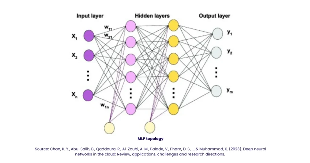
Architecture And Diagram of Multilayer Perceptron

When you imagine diagram of multilayer perceptron, visualize layers of nodes with arrows connecting them. A typical MLP structure:

Input layer (features) → Hidden layer(s) → Output layer

Each connection is associated with a weight, and each neuron has a bias term. Activation flows forward.

Here is a more descriptive version:

1. Input layer: passes the input features (e.g. x₁, x₂, x₃) to the network.
2. Hidden layer(s): neurons compute weighted sum + bias, then apply activation like ReLU or sigmoid.
3. Output layer: produces final prediction (e.g. class probabilities or regression output).

If we had one hidden layer with h neurons, and input dimension n, output dimension m, the weight matrices would be:

• of size : weights from input to hidden
• of size : biases in hidden
• Activation:
• Then output weights size , bias , output

If you draw arrows and nodes, that is your diagram of multilayer perceptron.

Because of space, I won’t insert a literal image, but imagine bubbles for neurons, arrows, and activation in between. Many tutorials show exactly such a diagram.

When you think of multilayer perceptron in machine learning, always visualize multiple hidden layers (or possibly just one) bridging input and output.

Learning In Multilayer Perceptron: Back Propagation

A key concept is back propagation in multilayer perceptrons. That is how the network learns to adjust weights to reduce error.

Forward pass

• You feed the network with an input.
• Each layer computes neuron outputs (weighted sum + bias, activation).
• Finally the output layer gives predictions .

You also know the true target values . You compute a loss function (e.g. mean squared error, cross-entropy) measuring difference between predictions and targets.

Backward pass (Backpropagation)

Back propagation is the process of propagating the error backward through the layers to adjust weights. The idea:

1. Compute error at the output:
   
2. For each hidden layer (from last hidden down to first hidden):
   
3. Weight updates:
   
   

Here is learning rate, is elementwise multiply, are activations from previous layer.

Thus using gradient descent and the chain rule, the network adjusts weights downward from output layer all the way to input connections. This is precisely back propagation in multilayer perceptrons.

One technical subtlety: the activation functions must be differentiable (so that exists). That is another reason we choose e.g. sigmoid, tanh, ReLU etc.

Because of this ability to propagate error through hidden layers, multilayer perceptron in machine learning can optimize weights across all layers.

Read More: Business Intelligence vs Data Analytics | Difference, Benefits & Careers

Why Backprop Matters

• It enables learning deep representations.
• It makes hidden layers meaningful (not just random).
• It handles large networks effectively (given enough compute, data, and smoothing).

Hence, multilayer perceptron in machine learning generally relies on back propagation in multilayer perceptrons as the standard training method.

An Example on XOR Gate Using Multilayer Perceptron

One classical illustrative example is xor gate using multilayer perceptron. XOR (exclusive OR) is not linearly separable, so a single perceptron fails. But a network with a hidden layer works.

XOR truth table

Input A	Input B	Output = A XOR B
0	0	0
0	1	1
1	0	1
1	1	0

As many tutorials say, a linear discriminant cannot separate these two classes in the plane. Thus, a single layer perceptron fails.

How MLP solves XOR

A small MLP with 2 input neurons, 2 hidden neurons, and 1 output neuron can implement XOR. Rough idea:

• Hidden layer neurons create internal features that are linear separations (e.g. one neuron learns “A OR B”, another learns “A AND B”).
• Output neuron combines hidden outputs to produce XOR target.

Because of hidden nonlinearity, the network can form the non-linear decision boundary needed.

This demonstrates the power of a multilayer perceptron in machine learning over single layer versions, and is often taught in introductory neural network courses.

Many use this example to show exactly back propagation in multilayer perceptrons at work.

Variants & Alternatives: Extreme Learning Machine for Multilayer Perceptron

So far we discussed the classical MLP with backpropagation. But there are variants and faster alternatives. One interesting variant is extreme learning machine for multilayer perceptron.

What Is Extreme Learning Machine?

Extreme Learning Machine (ELM) is a learning algorithm originally designed for single hidden layer feedforward networks (SLFNs). In ELM, input weights and hidden biases are randomly assigned, and only the output weights are computed analytically (via pseudoinverse). This makes the training extremely fast (hence “extreme”).

When you combine that idea into deeper networks, you get extreme learning machine for multilayer perceptron: extending random feature approach and analytic output layer solution to MLPs. Some research has explored hybrid schemes (random weights in some layers, backprop in others).

Pros and cons

Pros:

• Much faster training (no iterative weight updates for hidden layers)
• Simpler training pipeline
• Works well on small to medium datasets, in some cases surpassing backprop networks.

Cons:

• Less flexible (random initialization may not pick good hidden features)
• Not always competitive with deep backprop networks on complex tasks (e.g. image recognition).
• Harder to tune and generalize for many layers.

Thus, extreme learning machine for multilayer perceptron is an interesting approach if you prioritise speed and simplicity over maximal performance.

Strengths, Limitations and Tips

Let us now summarise multilayer perceptron in machine learning by looking at strengths, limitations, and some tips.

Strengths

• Can learn non-linear relationships
• Widely understood, with many libraries and tools
• Flexible: can be used for classification, regression, and many domains
• Well studied, with good theoretical foundations

Limitations

• Risk of overfitting, especially with many hidden units or layers
• Computationally expensive for large networks or datasets
• Requires proper hyperparameter tuning (learning rate, number of layers, neurons, activation)
• Sometimes “black box” – interpretability is low

Practical tips

• Start with a small network (1 hidden layer, few neurons), then scale
• Use regularisation (L2, dropout)
• Properly initialise weights (e.g. Xavier, He)
• Monitor training and validation loss to avoid overfitting
• Use suitable learning rate schedules
• Use cross-validation or holdout sets

Also, when designing architectures, visualize the diagram of multilayer perceptron and make sure connections and shapes are manageable.

Because the core training method is back propagation in multilayer perceptrons, ensure your loss is differentiable, activations are suitable, and gradients remain stable (watch out for vanishing or exploding gradients).

On A Final Note…

Here are the important takeaway points:

• Multilayer perceptron in machine learning is a feedforward neural network with hidden layers and nonlinear activation, enabling modelling of non-linear patterns.
• The question what is multilayer perceptron is answered by saying: it is a network of interconnected neurons arranged in multiple layers, trained via gradient methods.
• The difference between single layer and multilayer perceptron lies in representational power: the multilayer version can learn far more complex functions.
• The diagram of multilayer perceptron helps you visualise layers, nodes, weights and biases.
• Training uses back propagation in multilayer perceptrons: forward pass, error, backward pass, and weight updates via gradient descent.
• An illustrative case is xor gate using multilayer perceptron, showing why hidden layers matter.
• A variant is extreme learning machine for multilayer perceptron, which offers faster training by random hidden weights + analytic output weight solution.
• While potent, MLPs have limitations; careful tuning and design matters in practice.

FAQs